Locating Urban Scenes through Fine Tuning of Pre-trained Deep Learning Models
This is a summary of my group project done for the DATA7703 course for my Masters of Data Science study at the University of Queensland.
Geoguessr is a game where players are given a picture of a Google Street View imagery and try to guess where the image comes from. Players usually rely on man made features, like road markings or traffic signs to determine the location. Sometimes billboards come into play and show the language to narrow down possible locations. Although high level players like RAINBOLT have insane intuitions of colors and other features.. but I digress. But then, is it possible to create a bot that identifies the location of images by looking at the images?

There have been various efforts in identifying locations of pictures through machine learning, through location compression like GeoEstimation. The approach used in GeoEstimation is the classification of images to S2 cells which represent specific geographic boundaries on the surface of the earth. While this approach theoretically can be very accurate, it does raise some questions in regards to class relatedness (close areas should be more likely to be predicted) and the amount of labeled data we need. We want to reduce the scope to what would be useful in playing GeoGuessr, and also limit our training/input to dashcam-like images where images are captured onboard a vehicle, with mostly a view of the road ahead. Although Geoguessr does take geographic coordinates as an input for score, sampling down to the specific country is an easier output to do, and shifts the problem from classifying a photo to S2 cells, to photo -> country label.
When talking about image classification, most people would be thinking about classifying general objects, which is a problem that is quite popular and has been tackled by big teams with big resources. The first breakout Image Classification model using Neural Networks was the AlexNet, which needed to use the full ImageNet dataset which consists of 1.2 million images. The more recent improvements still also need at least that amount of training data, or even in the case of Vision Transformer, it uses 303 million images to train the model. Even if we have access to all of the images that Google Street View has, we probably don’t have the resources and time to train it.
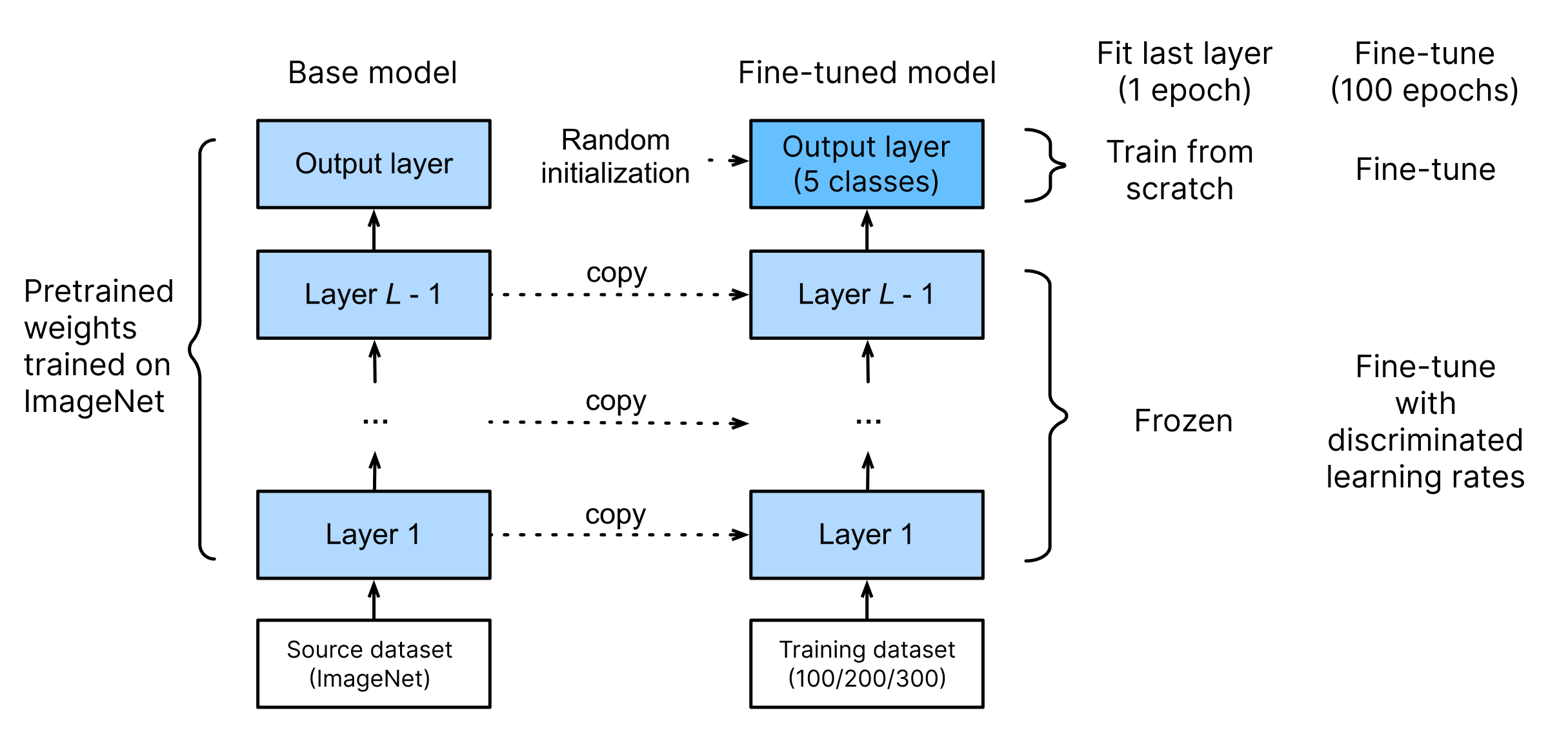
Fortunately, there’s a technique that can exploit the pre-trained general classification models for our own use, called Transfer Learning or Fine Tuning a model. Some prominent examples of this are the Stanford Dogs dataset, the Oxford Flowers-102 dataset, and the Stanford Cars dataset. For image classification tasks, the Fine Tuning process exploits the fact that the general classifiers have learned basic features of the images (as seen here), and we only need to change some parameters to use it for our specific problem, in this case classifying location based on features in the image.
We feel that the problem we are solving here is different to the usual fine-tuning problem as we are not trying to identify the same objects and classify them, and the objects of interest are not the main object of the image. Usual fine-tuning tasks have the main interest/class as the main object of the image, while classifying locations means having to identify unique, small features of the image to classify a single class, with varying amount of features and visibility for each class. We want to see how fine-tuning models fare in this regard.
As much as we’d love to use the Google Street View dataset, the access to it is paid, and that makes it not feasible to use. We instead found the Mapillary Traffic Sign dataset suitable for our use. It is a dataset that is compiled to train and evaluate object detection models for traffic signs. It is suitable for our use case as it consists mainly of forward-facing onboard images, and likely has man made features seen in the images. The Mapillary dataset needed some work to get the geographic data of lat, lon (scraping + API access). Once done, we can reverse geocode and list the available images by country. Due to the limited data available, we are classifying the top-5 available countries, which are AU, JP, US, BR, and DE. After data cleanup, we have max 300 training images and 40 test images per label, totalling 1500 training images and 200 test images.
| Country Code | Image Count | Country Code | Image Count | Country Code | Image Count | Country Code | Image Count |
|---|---|---|---|---|---|---|---|
| US | 1824 | IT | 192 | CN | 119 | RO | 58 |
| AU | 851 | CO | 188 | CL | 101 | AE | 56 |
| BR | 554 | IN | 180 | ID | 88 | MA | 56 |
| JP | 480 | MX | 174 | SE | 87 | DK | 54 |
| DE | 479 | NL | 168 | BE | 80 | NO | 49 |
| TH | 303 | GB | 162 | UA | 76 | TW | 47 |
| FR | 275 | ES | 136 | AT | 74 | EC | 46 |
| CA | 257 | AR | 130 | HU | 73 | CH | 45 |
| RU | 255 | PL | 127 | MY | 64 | VN | 43 |
| ZA | 222 | NZ | 124 | PE | 62 | PY | 42 |
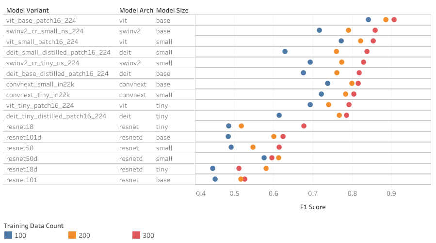
We are also interested in seeing how much data is needed to fine-tune to a specific problem, so we are fine-tuning the models with 100, 200, and 300 training images per label to see the difference.
To save time, we pre-resized the data to 800x800 pixels and squished it to a 1:1 aspect ratio. For the batch transformation, we used RandomResizedCropGPU to 224 pixels, brightness, and contrast augmentations. We do admit that this process is not optimum, and will touch on this later.
 For the model selection, Jeremy Howard has an evaluation of the Best vision models for fine tuning, and we’ll be using that as a basis. We feel that our specific problem has more similarity to the Kaggle Planet dataset in the evaluation. From this reference, we decided to evaluate ResNet, ResNet-d, ConvNExT, Vision Transformer (ViT), DEiT, and SWINv2. ResNet and ResNet d are chosen as the baseline models which are widely used for fine tuning use cases. ViT, ConvNext, DEiT and SWINv2 are chosen due to their good performance in the evaluation.
ResNet, ResNet-d, and ConvNExT are image classification models that uses convolutional architecture based on AlexNet and added Residual skip layers to enable deeper models. ResNet was the best performer when it was published and has been the default base of fine-tuned models. ResNet-D is an improved version of ResNet with some tricks. ConvNeXt applies lessons learned from Visual Transformers to convolutional neural networks to achieve similar performance.
Visual Transformer (ViT) is an image classification model based on the Transformer architecture that is predominantly used in Natural Language Processing tasks. Although it needs a lot of training data, it shows SOTA performance when it was published. DeiT is a Data Efficient variant of ViT that manages similar performance through modifications of architecture, training procedure and distillation. SWIN is a modified ViT by using hierarchical shifted windows to parse the image instead of just dividing the models to tokens.
For the model selection, Jeremy Howard has an evaluation of the Best vision models for fine tuning, and we’ll be using that as a basis. We feel that our specific problem has more similarity to the Kaggle Planet dataset in the evaluation. From this reference, we decided to evaluate ResNet, ResNet-d, ConvNExT, Vision Transformer (ViT), DEiT, and SWINv2. ResNet and ResNet d are chosen as the baseline models which are widely used for fine tuning use cases. ViT, ConvNext, DEiT and SWINv2 are chosen due to their good performance in the evaluation.
ResNet, ResNet-d, and ConvNExT are image classification models that uses convolutional architecture based on AlexNet and added Residual skip layers to enable deeper models. ResNet was the best performer when it was published and has been the default base of fine-tuned models. ResNet-D is an improved version of ResNet with some tricks. ConvNeXt applies lessons learned from Visual Transformers to convolutional neural networks to achieve similar performance.
Visual Transformer (ViT) is an image classification model based on the Transformer architecture that is predominantly used in Natural Language Processing tasks. Although it needs a lot of training data, it shows SOTA performance when it was published. DeiT is a Data Efficient variant of ViT that manages similar performance through modifications of architecture, training procedure and distillation. SWIN is a modified ViT by using hierarchical shifted windows to parse the image instead of just dividing the models to tokens.
| Base Architecture | Model Architecture | Tiny Variant | Small Variant | Base Variant |
|---|---|---|---|---|
| ResNet | ResNet | resnet18 (6M) | resnet50 (25M) | resnet101 (45M) |
| ResNet-d | resnet18d (6M) | resnet50d (25M) | resnet101d (45M) | |
| ConvNext | convnext-t (29M) | convnext-s (50M) | ||
| Visual Transformer (ViT) | ViT | vit-tiny (6M) | vit-small (22M) | vit-base (87M) |
| DEiT | deit-tiny (6M) | deit-small (22M) | deit-base (87M) | |
| SWINv2 | swinv2-tiny (28M) | swinv2-small (50M) |
All models will be fine tuned to 100 epochs with 1 epoch of last layer training. Ideal learning rate will be evaluated before the training. We’ll be evaluating the models through the accuracy_multi and f1_score metrics.
Results
 IMPACT OF TRAINING DATA AMOUNT
From the groph, it is clear that more data certainly helps any model to perform better. Using newer architectures such as ConvNext and ViT based architecture, the lack of data can be compensated by increasing the complexity of the model. Using 100 training images and tiny model variants limits the performance while using the same amount of training data and more complex models achieves similar performance to tiny models using more training data. This need for tiny models to train on a lot of data also shows the inverse. The newer tiny models can perform surprisingly well when trained with more data. The most flexible and resilient model seems to be ViT-Small and ViT-Base. It has a lower variance between 100-300 trained images and still achieves top 10 results in each case.
BEST PERFORMANCE
When a good amount of training data is available, the next consideration will be the size of the model and best performance available. Vit-base shows the best absolute performance here. Bigger sized model does not guarantee better performance, shown in the case of DeiT small vs base. Even though there is a significant improvement in each model variant, it has to be kept in mind that the unneeded complexity will impact in inference latency due to the size of the model.
 TRAINING THROUGHPUT
Bigger models need more time to fit, as shown in this graph. The impact from going to a vit-small model to Vit-Base model is roughly a 30% slower training period. It needs to be kept in mind that with 100 epochs, even the Vit-Base model only took around 35-40 minutes. The worst case model is the ConvNeXt models that takes around 1 hour to train for 100 epochs. This matters more in iterating the approach to the final model instead of having to wait for hours or days for the next model to evaluate.
INFERENCE THROUGHPUT
We took measurements of inference time from inference our test set. From the results we can see that the bigger models do have a latency penalty in inferencing. There is also a clear tradeoff between inference throughput and model performance, with 5% worse throughput and 5% better F1 Score by moving from Tiny models to Small models, and a further 10% worse throughput with 5% better F1 Score moving from Small models to Base models. ViT, SWINv2, and ConvNext models scale as expected while DEiT-Base achieves worse F1 Score compared to DEiT Small.
Conclusion
We believe that we have demonstrated that medium-complexity classification models can be created through fine-tuning/transfer learning techniques, with resources that are easily attainable by small teams or individuals. The results we get, with the best performing models having >0.9 F1 score on Base models and >0.85 F1 score on Small models, is clearly satisfactory. We have managed to do this with a reasonable amount of training dataset, with a maximum of 340 images per label, 300 training images and 40 test images per label. All of our training can be done with easily attainable resources, being done on 16GB GPU Paperspace machines (Free-RTX5000) that cost us USD 8 per month to access. If we are not evaluating many models, we can see more performant models through iterating on the training hyperparameters and data augmentation.
We also have proven that although various architectures are available and perform well, each specific classification task would need to evaluate several models to fit their needs. In general, newer models perform better through their architecture improvements. Small, newer models perform really well beyond expectations, so choosing them to start creating models is a good default. Although our best performing models are quite big on parameter size (ViT-Small 22M, Swinv2-Small 50M, ViT-Base 80M), there’s possible improvements coming through model compression such as MiniViT and TinyVit.
We have demonstrated that more images has a direct impact on the performance of the models, but the amount of data is not prohibitive. Although we have not exhaustively tested this, the amount of images that we tested reflects a possible range for other similarly difficult tasks. We also found that cleaning the data from irrelevant/low-quality images brings better performance, which matters more than the raw amount of data available.
An interesting point that we discover is that the ungeneralizable performance rankings of general image classification tasks such as ImageNet for specific classification tasks. From the published papers, ConvNext, DEiT, and SWINv2 have better performance than ViT of similar size in image classification tasks, but it is not the case here. It is possible that the larger size or inefficiency of the base ViT model has the extra space for the embedded knowledge needed for our specific classification tasks.
Next
Unfortunately we did not have time to dig deeper into the model and evaluate specifically how these models accomplish the classification. Some methods are available to evaluate these, like creating maximum activation images, attention maps or Transformer-specific interpretability techniques. We tried creating maximum activation images for some earlier ResNet models that we trained, but did not get satisfactory results.
Relatedly, there are improvements in the models that we use as the base models. There are improvements from the size constraints like MiniViT variants of DEiT and SWIN, also TinyViT. For performance and more robust learning, there’s also the modified RobustViT and RobustDeiT models that have been trained to learn from the object itself instead of background features, which we assume would perform better.
For the problem side, we wish to be able to evaluate the ultimate performance of classifier models, by training with more data and labels.